Estimating the maximum Bitcoin achievable via DCA - Part 1

Abstract: This article derives a mathematical formula for the amount of Bitcoin one can accumulate by following a continuous DCA strategy, assuming that Bitcoin’s price follows a Power Law. We will also derive a formula for the theoretical maximum amount of Bitcoin that can be owned by starting a DCA at a specific point in time.

Introduction

One of the most popular investment strategies in the Bitcoin space is Dollar-Cost Averaging (DCA). The approach is simple: invest a fixed amount of money at regular intervals, regardless of the price. This strategy helps to average out the purchase price over time and reduces the risk of buying at a market top.

A common question that arises is: how much Bitcoin can one accumulate using this strategy? The answer depends on the price evolution of Bitcoin. While predicting the exact price is impossible, we can use long-term models to get a reasonable estimate. One such model is the Power Law ¹, which suggests that Bitcoin’s price follows a predictable trajectory when viewed on a logarithmic scale over time.

This article derives a mathematical formula for the amount of Bitcoin one can accumulate by following a continuous DCA strategy, assuming that Bitcoin’s price follows a Power Law. We will also derive a formula for the theoretical maximum amount of Bitcoin that can be owned by starting a DCA at a specific point in time.

Tip: This article includes a simple calculator at the end to estimate your maximum potential Bitcoin stack. For a more feature-rich version that also allows for retirement income calculations, check out the Desmos app here.

Setup

To build our model, we first need to define our variables and state our assumptions.

Definitions

• $t$: Time measured in months (or weeks, days etc) since Jan 2009
• $t_0$: Start date of DCA
• $c$: Fixed dollar amount invested per unit time
• $k$: Power law exponent
• $P$: Price of Bitcoin at time $t$ (Average trend value)
• $A$: A fitting constant in the power law price model
• $N$: Amount of Bitcoin stacked at $t > t_0$
• $N_0$: Amount of Bitcoin at $t_0$

Model Assumptions

We begin by assuming that the price of Bitcoin, $P$, can be described by a simple Power Law model as a function of time, $t$: \begin{equation}\label{eq:power_law_price} P = A t^k \end{equation} Here, $A$ and $k$ are constants that can be determined by fitting the model to historical Bitcoin price data. The exponent $k$ captures the rate of price growth, while $A$ acts as a scaling factor. A key assumption here is that this model represents a long-term trend, deliberately smoothing out significant price volatility and cyclical patterns (e.g., 4-year halving cycles). The timing of DCA relative to these cycles can have a substantial impact on short-to-medium term accumulation, which is not captured in this analysis.

Initial Conditions

For this derivation, we assume that we start with no Bitcoin at the beginning of our DCA strategy. Therefore, the amount of Bitcoin at time $t_0$ is zero: \begin{equation}\label{eq:initial_condition} N_0 = 0 \quad \end{equation}

Derivation

With our setup complete, we can now derive the formula for the amount of Bitcoin accumulated over time.

I. Start by treating DCA as a continuous process

In a continuous DCA model, we invest an infinitesimally small amount, $c dt$, over an infinitesimally small time interval, $dt$. The incremental increase in our Bitcoin stack, $dN$, is this invested amount divided by the price, $P$, at that time. This relationship is expressed in the following differential equation: \begin{equation}\label{eq:dca_continuous} dN = \frac{c}{P} dt \end{equation}

Note: The infinitesimally small time interval $dt$ is used to enable calculus-based derivation. This continuous model should approximate real-world DCA well, provided the investment frequency is at least monthly, as the price changes between consecutive investments would be relatively small.

Next, we substitute the Power Law price model from Equation \eqref{eq:power_law_price} into Equation \eqref{eq:dca_continuous} to describe the incremental accumulation in terms of time: \begin{equation}\label{eq:dca_price_substituted} dN = \frac{c}{A t^k} dt \end{equation}

II. Integrate the equation

To find the total amount of Bitcoin, $N$, accumulated from a start time $t_0$ to a future time $t$, we integrate Equation \eqref{eq:dca_price_substituted}. We integrate the left side from our initial holding $N_0$ to the final holding $N$, and the right side from time $t_0$ to $t$: \(\begin{align} \int_{N_0}^{N} dN &= \int_{t_0}^{t} \frac{c}{A t^k} dt \label{eq:integral_setup} \\ \Rightarrow N - N_0 &= \frac{c}{A} \int_{t_0}^{t} t^{-k} dt \\ \Rightarrow N &= N_0 + \frac{c}{A(1-k)} \left[ t^{-k+1} \right]_{t_0}^{t} \label{eq:integrated} \end{align}\) Applying our initial condition from Equation \eqref{eq:initial_condition} where $N_0=0$, the equation simplifies to: \begin{equation}\label{eq:accumulated_btc_raw} N = \frac{c}{A(1-k)} \left( t^{1-k} - t_0^{1-k} \right) \end{equation} After rearranging the terms to make the expression more intuitive (assuming $k > 1$), we arrive at the final formula for the amount of Bitcoin accumulated: \begin{equation}\label{eq:accumulated_btc_final} N = \frac{c}{A(k-1)} \left( \frac{1}{t_0^{k-1}} - \frac{1}{t^{k-1}} \right) \end{equation}

III. Maximum Bitcoin Estimation

A fascinating consequence of this model is that it predicts a theoretical maximum amount of Bitcoin that can be accumulated. To find this maximum, $N_{max}$, we take the limit of Equation \eqref{eq:accumulated_btc_final} as time $t$ approaches infinity. \(\begin{align} N_{max} &= \lim_{t \to \infty} \frac{c}{A(k-1)} \left( \frac{1}{t_0^{k-1}} - \frac{1}{t^{k-1}} \right) \label{eq:max_btc_limit} \\ &= \frac{c}{A(k-1)} \left( \frac{1}{t_0^{k-1}} - 0 \right) \end{align}\) The term $\frac{1}{t^{k-1}}$ approaches zero as $t \to \infty$ (assuming $k > 1$, which is true for Bitcoin’s historical price). This leads to the final expression for the maximum amount of Bitcoin that can be accumulated: \begin{equation}\label{eq:max_btc_final} N_{max} = \frac{c}{A(k-1)t_0^{k-1}} \end{equation} This result is profound. It implies that for a given investment rate, the maximum amount of Bitcoin one can ever accumulate is predetermined by the time one starts investing ($t_0$). The earlier you start, the larger your potential maximum stack.

Analysis

Determining the constants $k$ and $A$

The formula for the maximum amount of Bitcoin that can be accumulated requires two parameters to be determined: the power law exponent $k$ and the constant $A$. They are determined by fitting the power law model to the historical price of Bitcoin. Below are the values I used for the calculations in this article:

• $k = 5.7$
• $A = \exp(-38.184)$, for time measured in days.

Impact of investment rate $c$

Below is the chart showing the Bitcoin accumulation over time starting from Jan 2025 for various monthly investment amounts. As you can see, the amount of Bitcoin stacked rapidly increases at first, but eventually plateaus to a terminal value over time.

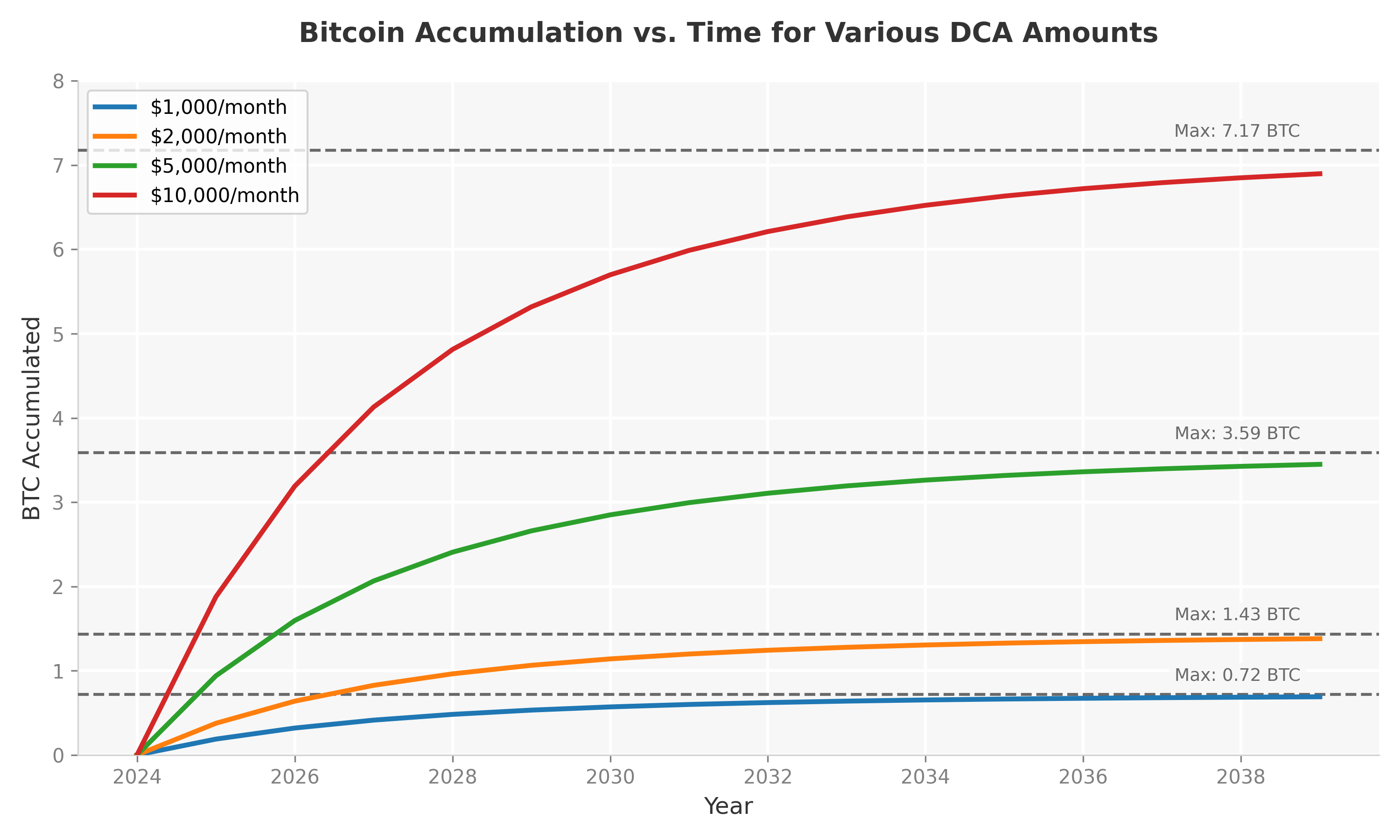Figure 1: Bitcoin accumulation curves for different monthly DCA amounts, starting in 2024.

Impact of starting time $t_0$

In addition to the dollar amount invested, the starting time $t_0$ also plays a crucial role. Below is the chart showing the Bitcoin accumulation over time starting from Jan 2025 for various starting times.

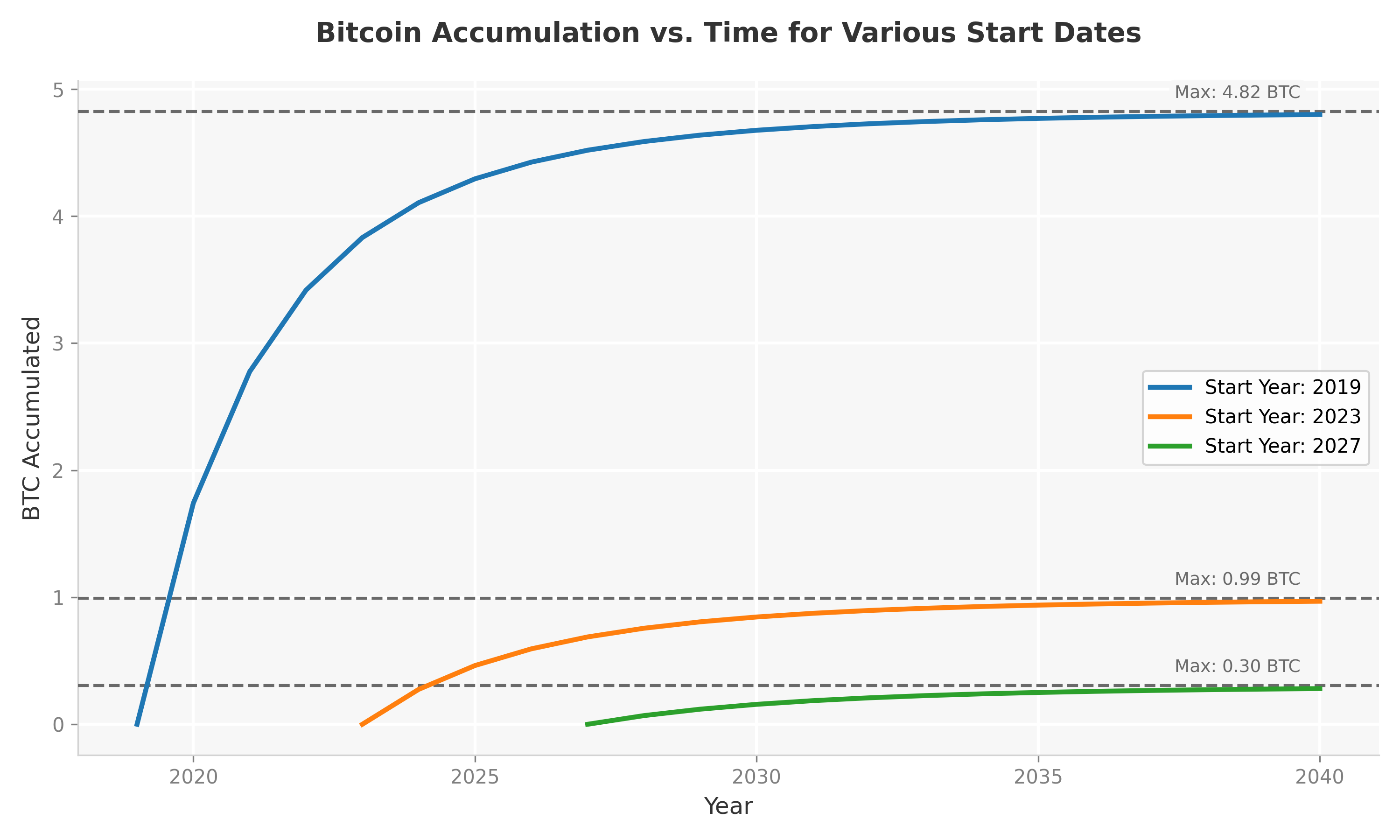Figure 2: Bitcoin accumulation for a $1,000/month DCA, showing the impact of different start dates.

The Maximum Bitcoin Contours

Achieving the mythical 1 Bitcoin is a popular goal for many Bitcoiners. This feat is becoming increasingly difficult as the price growth of Bitcoin accelerates. This is illustrated in the contour plot below, where the contours represent the maximum amount of Bitcoin that can be accumulated for different starting times and investment rates.

Figure 3: Maximum BTC accumulated for different starting years and monthly DCA amounts.

The chart clearly shows the difficulty of achieving a certain amount of Bitcoin, especially as time progresses. For instance, a family earning \$100,000 per year that DCAs into Bitcoin starting 2025 will need to put aside about 24% of their income or \$24,000 per year every year into Bitcoin to get close to 1 BTC. That same family would need to put a whopping 84% of their income i.e. \$84,000 per year into Bitcoin if they instead started five years later in 2030 to achieve the same stack.

Conclusion and Further Exploration

In this article, we derived a set of formulas to model Bitcoin accumulation via a continuous Dollar-Cost Averaging strategy, based on a Power Law price model. Our derivation produced an equation for the amount of Bitcoin accumulated over a given period, and more importantly, a formula for the theoretical maximum amount of Bitcoin one can acquire, which is inversely proportional to the start time raised to the power of $k-1$.

This analysis opens up several avenues for further exploration:

• Data Validation: Before refining the model, a crucial first step is to rigorously backtest the existing model to see how well its predictions have matched historical accumulation outcomes. This helps to quantify the model’s accuracy and its limitations.
• Model Calibration: Based on the validation results, one could perform a fresh regression on historical Bitcoin price data to find the optimal values for the constants $A$ and $k$.
• Impact of Price Cycles: A major simplification in this article is the exclusion of Bitcoin’s well-known price cycles. A more advanced and highly important analysis would study how the phase of the cycle at the start of a DCA strategy impacts the total accumulated Bitcoin. For instance, starting a DCA during a bear market versus a bull market would yield significantly different results, a factor not considered here.
• Sensitivity Analysis: It would be insightful to analyze how sensitive the accumulated amount of Bitcoin is to changes in the investment rate $c$, the power law exponent $k$, and the starting time $t_0$.
• Discrete vs. Continuous DCA: Our model assumes continuous investment. A more practical analysis could explore a discrete DCA model (e.g., weekly or monthly investments) and compare the results to the continuous case.

By providing a mathematical framework for understanding DCA in the context of Bitcoin’s long-term growth, we can gain a deeper appreciation for the dynamics of accumulation and the importance of starting early.

Calculator

Below is a simple calculator that allows you to estimate the maximum amount of Bitcoin that can be accumulated based on your monthly investment amount. For a more feature-rich calculator that also allows retirement income calculations, check out my Desmos app here.

DCA Max Bitcoin Estimator

Enter your monthly DCA amount to estimate the theoretical maximum Bitcoin you could accumulate if you start today.

Monthly DCA Amount (USD):

References

1. Wheatley, S., Sornette, D., Huber, T., Reppen, M., & Gantner, R. N. (2018). Are Bitcoin Bubbles Predictable? Combining a Generalized Metcalfe’s Law and the LPPLS Model. SSRN Electronic Journal. ↩︎