The Bitcoin Flow Equation - A Mathematical Prelude

Abstract: This article introduces the Bitcoin Flow Equation (BFE), a mathematical framework for modeling Bitcoin portfolios with active cashflow strategies. It provides a unified model of Bitcoin price and cashflow that enables new financial planning paradigms. The BFE is a powerful tool for strategic planning, allowing you to develop a custom income generation strategy based on your financial goals and risk tolerance. It also allows you to calculate the required fixed investment rate to reach a specific portfolio value by a future time. Leverage can be modeled by treating the loan as a large initial positive cashflow, and the interest and principal payments as a negative cashflow. The BFE can help analyze the risks and potential returns of such a strategy.

Definitions

• $S$: The value of the Bitcoin portfolio in dollars.
• $N$: The number of Bitcoin in the portfolio.
• $P$: The price of Bitcoin in dollars.
• $C$: The net cashflow in dollars.
• $dt$: The small change in time.
• $dS$: The small change in the value of the portfolio in dollars.
• $k$: The power law exponent.

Introduction

Bitcoin’s price power law provides a robust model for understanding the asset’s long-term growth trajectory¹. However, it alone is insufficient for modeling real-world Bitcoin portfolios. It is only useful for scenarios involving one-time purchases and sales of Bitcoin over a given period. However, in practice, Bitcoin portfolio management is a continuous process of buying and selling. Consider dollar-cost averaging (DCA), a popular strategy where investors regularly purchase fixed dollar amounts of Bitcoin. In such cases, the portfolio’s value follows a more complex trend that combines both the power law price growth and the gradual accumulation of Bitcoin holdings. The Bitcoin Flow Equation (BFE) addresses this complexity by providing a mathematical framework for modeling Bitcoin portfolios with active cashflow strategies.

This article is a prelude to a more detailed article on the Bitcoin Flow Equation. Here I will give a brief mathematical introduction to the core idea.

Lets say you want to model the change in value of a Bitcoin portfolio over time. Let this be represented by the symbol $S$. If the portfolio has $N$ Bitcoin and $P$ is the price of Bitcoin then \begin{equation} S=PN \label{eq:1} \end{equation}

The change in value of the portfolio is a combination of both the change in price of Bitcoin and the change in the number of Bitcoin in the portfolio. This can be expressed by the following differential equation: \begin{equation} dS = dPN+PdN \label{eq:dS1} \end{equation} Here $dS$ is a small change in value of the portfolio, $dP$ is a small change in price of Bitcoin and $dN$ is the incremental number of Bitcoin bought at a price $P$. The term $PdN$ gives the incremental cashflow. Lets represent this with the symbol $dC$. Furthermore, from equation \ref{eq:1} we have $dN = \frac{dS}{P}$. Combining both these definitions, we get:

\begin{equation} dS = \frac{dP}{P}S+dC \label{eq:2} \end{equation}

Equation \ref{eq:2} sets the stage for the introduction of the Bitcoin Flow Equation (BFE). The next step is to introduce a model for the price and the cashflow process that enables us to solve for $S$ and derive valuable insights. This is the subject of the remainder of this article.

Modeling Price and Cashflow

Price Model

The power law model gives the simplest, most robust prediction of Bitcoin’s long-term price trend as a function of its age $t$ ². A general form of the power law is: \begin{equation} P(t) = At^k \label{eq:3} \end{equation} where $A$ is a constant and $k$ is the power law exponent. The values of $A$ and $k$ are estimated by fitting the power law model to historical Bitcoin price data. Empirically, $k$ has been observed to be around 5.6-5.8 depending on the time period and methodology used to estimate it.

For our continuous model, we need the differential form. Taking the derivative with respect to time gives: \begin{equation} dP = kAt^{k-1}dt \label{eq:4} \end{equation} Dividing equation \ref{eq:4} by equation \ref{eq:3} gives: \begin{equation} \frac{dP}{P} = k\frac{dt}{t} \label{eq:5} \end{equation} Plugging this into equation \ref{eq:2} gives: \begin{equation} dS = k\frac{S}{t}dt + dC \label{eq:6} \end{equation} Dividing both sides by $dt$ gives: \begin{equation} \boxed{\quad\vphantom{\Bigg|}\displaystyle\frac{dS}{dt} = k\frac{S}{t} + \frac{dC}{dt}\quad\vphantom{\Bigg|}} \label{eq:7} \end{equation} The above equation is henceforth termed the Bitcoin Flow Equation (BFE). It states that the rate of change of the Bitcoin portfolio value can be expressed as the sum of the power law growth rate $k\frac{S}{t}$ and the cashflow rate $\frac{dC}{dt}$.

Cashflow Process

Depending on the strategy, there are several ways to model the cashflow process.

• Fixed Cashflow: $\frac{dC}{dt} = constant$. This models a constant rate of investment like dollar cost averaging or conversely a fixed income strategy.
• Power Law Cashflow: $\frac{dC}{dt} = bt^m$. This could model an investment strategy that ramps up or down over time. Here $b$ is a constant and $m$ is the power law exponent.
• Time-Adjusted Proportional Cashflow: $\frac{dC}{dt} = \alpha\frac{S}{t}$. Here, the cashflow rate is a fraction of the portfolio’s value, adjusted by time in order to account for the diminishing returns of the power law model. This can shown to be useful for modeling withdrawal strategies that enable a predictable Bitcoin stack that is robust to price volatility.
• Leveraged Cashflow: $\frac{dC}{dt} = \gamma\frac{dS}{dt}$. This models leveraged strategies with a fixed LTV given by $\gamma$. Here, cashflow is generated from the change in the portfolio’s value. When the portfolio value increases, the investor is able to borrow against the appreciation to generate cashflow.

Solving the Equation

The General Solution

To solve the equation, we first rearrange it into the standard form for a linear first-order ODE: \begin{equation} \frac{dS}{dt} - \frac{k}{t}S = \frac{dC}{dt} \end{equation} We can solve this using an integrating factor, $I(t) = t^{-k}$. Multiplying the equation by $I(t)$ gives: \begin{equation} t^{-k}\frac{dS}{dt} - kt^{-k-1}S = t^{-k}\frac{dC}{dt} \end{equation} The left side is the derivative of $S \cdot t^{-k}$: \begin{equation} \frac{d}{dt}(S \cdot t^{-k}) = t^{-k}\frac{dC}{dt} \end{equation} To find a particular solution, we integrate from a starting time $t_0$ to a future time $t$. Let’s assume we start with an initial capital $S_0$ at time $t_0$, so $S(t_0) = S_0$. \begin{equation} \int_{t_0}^{t} \frac{d}{d\tau}(S(\tau) \cdot \tau^{-k})d\tau = \int_{t_0}^{t} \tau^{-k}\frac{dC}{d\tau}d\tau \end{equation} \begin{equation} S(t)t^{-k} - S_0t_0^{-k} = \int_{t_0}^{t} \tau^{-k}\frac{dC}{d\tau}d\tau \end{equation} This yields the general solution for $S(t)$ in terms of the initial conditions: \begin{equation} \boxed{\quad\vphantom{\Bigg|}S(t) = S_0\left(\frac{t}{t_0}\right)^k + t^k \int_{t_0}^{t} \tau^{-k}\frac{dC}{d\tau}d\tau\quad\vphantom{\Bigg|}} \end{equation} This solution beautifully separates the final value into two components:

1. $S_0(t/t_0)^k$: The growth of your initial capital, $S_0$.
2. $t^k \int_{t_0}^{t} \tau^{-k}\frac{dC}{d\tau}d\tau$: The future value of all cashflows made between $t_0$ and $t$.

Fixed Cashflow

Let’s solve for the simplest case, where $\frac{dC}{dt} = c_0$ is a constant. The integral term becomes: \begin{equation} \int_{t_0}^{t} \tau^{-k}c_0 d\tau = \frac{c_0}{1-k}(t^{1-k} - t_0^{1-k}) \end{equation} Substituting this back into the general solution gives: \begin{equation} S(t) = S_0\left(\frac{t}{t_0}\right)^k + \frac{c_0}{1-k}(t - t_0^{1-k}t^k) \end{equation} This equation tells you the value of your holdings at any time $t$, given an initial investment $S_0$ and a constant cashflow rate $c_0$.

For positive values of $c_0$, this represents the well known dollar cost averaging strategy. For negative values of $c_0$, this represents a fixed income strategy. Within income generation strategies, there are three variations depending on the magnitude of $c_0$.

• Underdraw - $c_0 > \frac{S_0(1-k)}{t_0}$: Income is generated, however the portfolio value will still grow at a nonlinear rate.
• Critical Draw - $c_0 = \frac{S_0(1-k)}{t_0}$: The withdrawal rate is just high enough that your portoflio still grows, albeit at a very slow linear rate. Any further increase in the withdrawal rate will cause the portfolio to shrink.
• Overdraw - $c_0 < \frac{S_0(1-k)}{t_0}$: The withdrawal rate is so high that the price growth is not enough to compensate for the reduction in the portfolio value. Thus, the portfolio will shrink over time.

In the following Twitter/X thread, I explored the special case of the critical draw and showcased how income generated as a function of the portfolio value and retirement age.

The #Bitcoin water well💧

1/5
Once constructed, a water well is a continuous source of free drinking water that gets naturally replenished over time. However, if consumed too quickly, the well dries up and the village goes thirsty.

Similarly, since bitcoin is a continuously… pic.twitter.com/iUteTCuUN2

— Ashwin (@metashwin) July 12, 2024

I have also created a Desmos app based on the fixed cashflow model that allows you to plan your Bitcoin accumulation and income generation strategies - Bitcoin Water Well - v1.

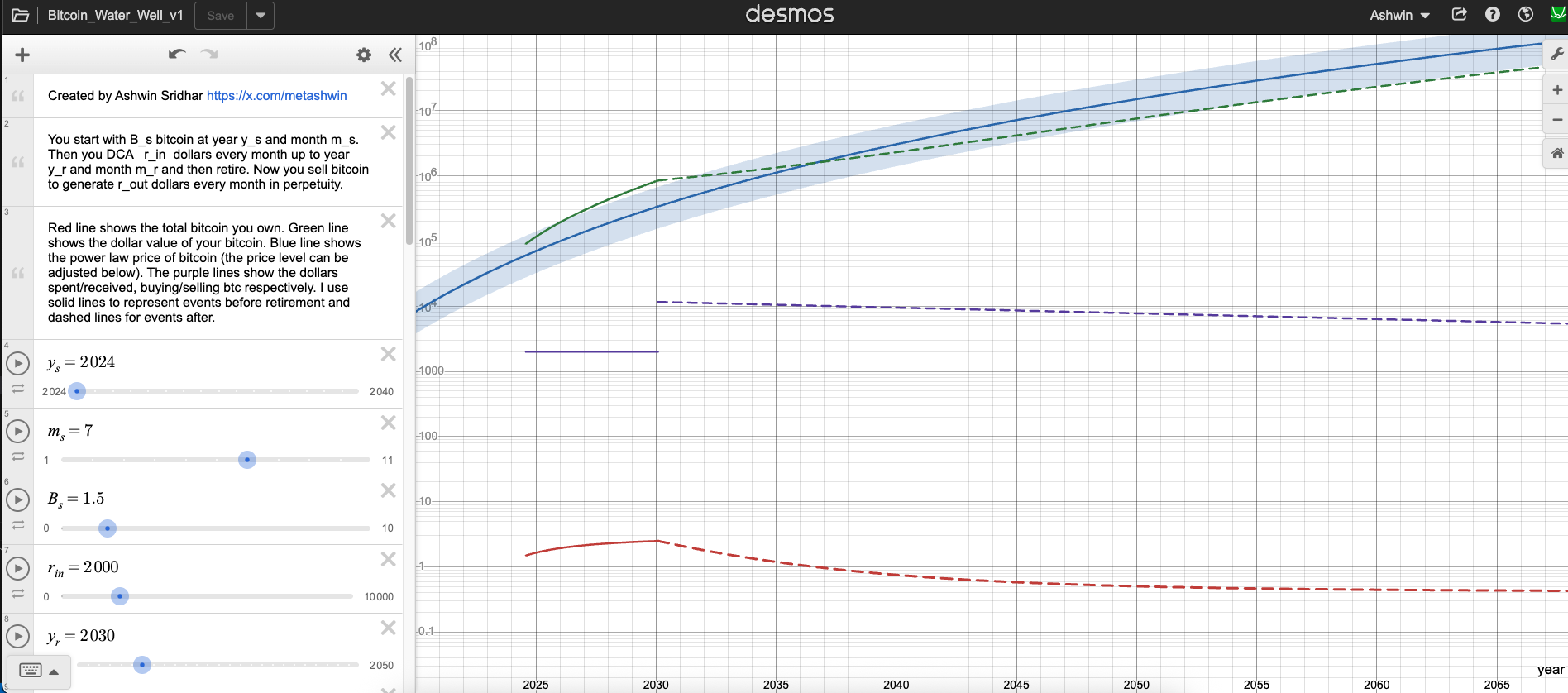Figure 1: Screenshot of the Desmos Bitcoin Water Well app, which allows you to explore accumulation and income strategies under the fixed cashflow BFE model.

Power Law Cashflow

Now consider a variable cashflow, $\frac{dC}{dt} = bt^m$. The integral is: \begin{equation} \int_{t_0}^{t} \tau^{-k}(b\tau^m)d\tau = \frac{b}{m-k+1}(t^{m-k+1} - t_0^{m-k+1}) \end{equation} Assuming $m-k+1 \neq 0$, the solution is: \begin{equation} S(t) = S_0\left(\frac{t}{t_0}\right)^k + \frac{b}{m-k+1}(t^{m+1} - t_0^{m-k+1}t^k) \end{equation} This allows for modeling more complex strategies where your investment or withdrawal rate changes over time according to a power law. For example, lets say instead of retiring in one go, you want to slowly transition into it by ramping up your cashflow over time. This can be modeled by setting $m=1$, which results in a linearly increasing income stream starting from zero at the start of retirement. Adjusting the parameter $b$ allows to control the slope of the ramp.

Time-Adjusted Proportional Cashflow

This strategy is particularly useful for modeling withdrawals. The cashflow rate is set to be a fraction of the portfolio’s value, adjusted by time: $\frac{dC}{dt} = \alpha\frac{S}{t}$. Here, $\alpha$ is a constant, which would be negative for withdrawals. Let’s substitute this into the BFE: \begin{equation} dS = k\frac{S}{t}dt + \left(\alpha\frac{S}{t}\right)dt \end{equation} We can combine the terms on the right-hand side: \begin{equation} dS = (k+\alpha)\frac{S}{t}dt \end{equation} This is a separable differential equation. \begin{equation} \frac{dS}{S} = (k+\alpha)\frac{dt}{t} \end{equation} Integrating both sides and using the initial condition $S(t_0)=S_0$ yields a simple power law, but with a modified exponent: \begin{equation} S(t) = S_0\left(\frac{t}{t_0}\right)^{k+\alpha} \end{equation} The key advantage of this withdrawal strategy is that the amount of Bitcoin in the portfolio follows a simple, predictable power law, To see this, let’s consider the amount of Bitcoin in the portfolio, $N(t) = S(t)/P(t)$. Since $P(t) = P_0(t/t_0)^k$, we get: \begin{equation} N(t) = \frac{S_0\left(\frac{t}{t_0}\right)^{k+\alpha}}{P_0\left(\frac{t}{t_0}\right)^k} = \frac{S_0}{P_0}\left(\frac{t}{t_0}\right)^{\alpha} = N_0\left(\frac{t}{t_0}\right)^{\alpha} \end{equation} Compared to a fixed cashflow withdrawal which leads to selling a disproportionately large amount of Bitcoin early on, this method provides a more determinate and smoother rate of selling over time that is also more robust to price volatility. This will be explored in more detail in a future article.

Leveraged Cashflow

In this model, the cashflow is proportional to the change in the portfolio’s value: $\frac{dC}{dt} = \gamma\frac{dS}{dt}$. The parameter $\gamma$ represents the Loan-to-Value (LTV) ratio. You borrow against your portfolio’s appreciation to generate cashflow, effectively amplifying your investment.

Substituting the leveraged cashflow rate into the BFE gives: \begin{equation} dS = k\frac{S}{t}dt + \left(\gamma\frac{dS}{dt}\right)dt \end{equation} \begin{equation} dS(1-\gamma) = k\frac{S}{t}dt \end{equation} \begin{equation} \frac{dS}{S} = \frac{k}{1-\gamma}\frac{dt}{t} \end{equation} Integrating this equation shows that this strategy effectively modifies the power law exponent. Solving for $S(t)$ and using the initial condition $S(t_0) = S_0$ yields: \begin{equation} S(t) = S_0\left(\frac{t}{t_0}\right)^{\frac{k}{1-\gamma}} \end{equation} This powerful result shows how leverage increases the power law exponent, amplifying returns.

Use Cases of the Bitcoin Flow Equation

The BFE is a powerful tool for strategic planning.

• Income Generation: It allows you to develop a custom income generation strategy based on your financial goals and risk tolerance.
• Accumulation Targets: You can calculate the required fixed investment rate to reach a specific portfolio value by a future time.
• Leverage Strategies: Leverage can be modeled by treating the loan as a large initial positive cashflow, and the interest and principal payments as a negative cashflow. The BFE can help analyze the risks and potential returns of such a strategy.
• Studying Synthetic Power Laws: The BFE allows for the creation and study of synthetic power laws. This is particularly relevant for analyzing entities like Bitcoin treasury companies. For instance, MicroStrategy, which holds the largest corporate Bitcoin treasury, is already showing signs of following its own power law (see Figure 2). The BFE can reveal how this trajectory is connected to its cashflow generation and leverage ratio.

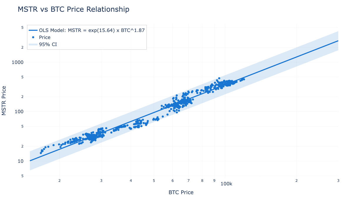Figure 2: MicroStrategy vs Bitcoin price shows a clear power law with an exponent of 1.87. The BFE framework could potentially shed a light on how such a relationship can emerge from an underlying leveraged cashflow process.

Next Steps

This prelude provides the basic framework. Future articles will delve deeper into specific examples, historical backtesting, and the implications of this model by exploring the following:

• Incorporate More Sophisticated Price Models: The current model uses a simple power law, but more advanced models could include cyclical components or stochastic elements to represent volatility. This would provide a more realistic price path for backtesting strategies and understanding short-term risks.
• Explore Each Cashflow Process in Detail: Each cashflow type—fixed, power law, and time-adjusted—deserves a dedicated analysis with practical examples and visualizations. This would help build intuition for how each strategy behaves under different market conditions and for different financial goals.
• Compare Withdrawal Strategies: A detailed comparison of fixed, ramp, and time-adjusted withdrawal strategies could show the pros and cons of different ways to generate income. This analysis would provide a clear guide for retirees or others looking to live off their Bitcoin investments.
• Model Interest Payments for Leveraged Cashflow: A more realistic model of leverage must account for the cost of borrowing. This involves incorporating interest payments as a negative cashflow component, allowing for a more accurate assessment of the net returns and risks of leveraged strategies.
• Apply the Kelly Criterion to Rebalancing Strategies: The Kelly criterion is a formula used to determine the optimal size of an investment to maximize long-term growth. We can adapt this framework to find the optimal rebalancing or leverage ratio within the BFE context, helping to maximize growth while managing risk.
• Add a Dollar Cash Balance as a State Variable: Tracking the dollar cash balance separately would allow for more complex financial planning. This enables modeling scenarios where cash from sales is accumulated and redeployed later, making the BFE a more complete financial planning tool.
• Perform Data Validation Studies: To build confidence in the BFE, its predictions should be tested against Bitcoin’s actual price history. This involves running simulations of different strategies using historical data to identify the model’s limitations and refine its parameters for better accuracy.
• Analyze treasury companies: Apply the BFE lens to analyze the cashflow and leverage of treasury companies like MicroStrategy.

References

1. Wheatley, S., Sornette, D., Huber, T., Reppen, M., & Gantner, R. N. (2018). Are Bitcoin Bubbles Predictable? Combining a Generalized Metcalfe’s Law and the LPPLS Model. SSRN Electronic Journal. ↩︎

2. Burger, H. C. (2019). Bitcoin’s natural long-term power-law corridor of growth. Quantodian: Tracking Bitcoin. ↩︎